ComtradR unofficial tutorial
The UN Comtrade is a central provider of data for governments, academia, research institutes, and enterprises. This tutorial is for students and researchers who need to get started downloading data from the UN Comtrade database, with the intention of using R and RStudio for data processing. Note that the UN Comtrade also has its own Statistics wiki with an FAQ for first time users
Check out the R packages required for the prosess section for further information, including how to do the Technical preparations of the project. I, the author is a librarian and political scientist with many years of experience guiding and teaching in library use for students and researchers of political science. I am making this tutorial as part of my own effort in becoming a more digitally updated employee for my organization.-.-
Note
This text has incomplete references. References will be added at a later stage. Thanks to ropensci/comtradr for making the package available again. Thanks to Zotero.org for providing the LaTeX format
—
01 Data from Comtrade to RStudio
This is a tutorial for learning how to download Comtrade data and processing them in RStudio. It will be shown how data from the United Nations’ Comtrade database [@CRANPackageComtradr] can be used to point out variations in the export of crude oil from OPEC countries. This will be the example used to demonstrate both the process of data collection, as well as the parsing, processing and facilitation of data into relevant units. While working on this project, the United Nations API delivery was modernized and changed from being facilitated for R and RStudio into Python. The ComtradR is now maintained under the GitHub initiative of OpenSci[@muir2023; @ROpenSciOpenTools]. This project will be developed according to the progress of the technical development of the official Comtrade database. A repository on how to generate data with Python, for import to RStudio may come at a later time.
02 The problem of discussion
The tutorial will not bring you into rocket science. However, it may be used by people who need an example at how to download data. Problems of discussion will be kept simple. We will look at the OPEC countries and their oil export in crude oil. The time period we are going to analyze is 1995-2024. Data on Trade value in Crude oil will be collected from Comtrade legacy database [@muir2023]. “Trade value” was chosen because it is the variable in this category that includes the most data. If choosing another category, the number of missing values would have been larger. The development of the values of Trade value will be shown from the period 1995-2014. The steps from collecting to breaking down the data will be shown in a sequence that will be possible for a beginner to reconstruct.
03 Hypotheses
We are going to look at data from the Comtrade database published by the World bank.
Q1 What does the distribution of Export of Crude oil from the OPEC countries look like for the years from 1995 until today?
Q2 What does the available corruption index of the OPEC countries look like?
Q3 Is there a tendency for the OPEC countries that higher income from oil exports leads to higher levels of corruption?
04 A good way to start up an R script
If you do not know your directory, use the command “getwd”. Then, copy the directory from the answer you got, and adjust it to fit the path that suits you. In the .R file, at the very begining:
getwd
setwd("/Users/ragnhildsundsbak/Documents/LearningR2023/ComtradeProjectNew")
It is always start with the setwd. It is a good idea to combine it with opening the library(here). Many people prefer to use projects in RStudio. The reason why I no not, is that i feel the setwd command and “here” package gives me both better knowledge and control over my system.
In order to follow the process in this script, we need the following pagkages. Note that if you do not have them installed, you must first use the command install.packages(“package name”). Since this is to be done only once, I often use the # tag to make the coding turn into a comment that will not be executed.
1 Installation example:
install.packages("comtradr")
install.packages("rjson")

after installation, change to:
#install.packages("comtradr")
#install.packages("rjson")
2:
library(here)
library(comtradr)
library(rjson)
library(ggplot2)
library(dplyr)
library(plotly)
library(conflicted)
library(janitor)
library(tidyverse)
library(scales)

Selected output console:

> library(conflicted)
> library(janitor)
> library(tidyverse)
── Attaching core tidyverse packages ─────────── tidyverse 2.0.0 ──
✔ forcats   1.0.0     ✔ stringr   1.5.0
✔ lubridate 1.9.2     ✔ tibble    3.2.1
✔ purrr     1.0.1     ✔ tidyr     1.3.0
✔ readr     2.1.4
It is also necesary to rule out the conflicts between the packages that are in use 3:
conflict_scout()
4:
conflicts_prefer(stats::chisq.test)
conflicts_prefer(scales::col_factor)
conflicts_prefer(scales::discard)
conflicts_prefer(stats::filter)
conflicts_prefer(stats::fisher.test)
conflicts_prefer(stats::lag)
conflicts_prefer(plotly::layout)

Selected output:

> conflicts_prefer(scales::discard)
[conflicted] Will prefer scales::discard over any other package.
> conflicts_prefer(stats::filter)
[conflicted] Will prefer stats::filter over any other package.
> conflicts_prefer(stats::fisher.test)
[conflicted] Will prefer stats::fisher.test over any other
package.
> conflicts_prefer(stats::lag)
[conflicted] Will prefer stats::lag over any other package.
> conflicts_prefer(plotly::layout)
[conflicted] Will prefer plotly::layout over any other package.
>
We are ready to start the process of getting data.
04 Getting the data
The Comtrade database has different subscription levels. If you are fortunate enough to belong to an academic institution that has a subscription, you may use the Premium Pro API solution. If not, there is a possibility of using the free API solution. You may get more information in the FAQ for first time users: https://unstats.un.org/wiki/pages/viewpage.action?pageId=125141443
In order to get access to the API through RStudio We need to log into the Comtrade system. Read the New Comtrade User Guide and especially under the section “Developer portal”. Decide the correct user level or “Product” as they are called.
Use this path in order to navigate to the page of the promary key of your subscription: https://comtradeplus.un.org/ –> login –> My comtrade premium –> My API portal –> Sign in –> Profile and then you are there. As you can see, you must first log on to the Comtrade, and then log in again to the API solution on the small button named “Azure Active Directory B2C”.
5:
#From the logon page uio user
set_primary_comtrade_key()
The function defined in this example, get.Comtrade(), extracts data from UN Comtrade using either the csv or the json format. 6:
get.Comtrade <- function(url="http://comtrade.un.org/api/get?"
                      ,maxrec=50000
                      ,type="C"
                      ,freq="A"
                      ,px="HS"
                      ,ps="now"
                      ,r
                      ,p
                      ,rg="all"
                      ,cc="TOTAL"
                      ,fmt="json")
{string<- paste(url
              ,"max=",maxrec,"&" #maximum no. of records returned
              ,"type=",type,"&" #type of trade (c=commodities)
              ,"freq=",freq,"&" #frequency
              ,"px=",px,"&" #classification
              ,"ps=",ps,"&" #time period
              ,"r=",r,"&" #reporting area
              ,"p=",p,"&" #partner country
              ,"rg=",rg,"&" #trade flow
              ,"cc=",cc,"&" #classification code
              ,"fmt=",fmt        #Format
              ,sep = "")
if(fmt == "csv") {
    raw.data<- read.csv(string,header=TRUE)
    return(list(validation=NULL, data=raw.data))
} else {
 if(fmt == "json" ) {
   raw.data<- fromJSON(file=string)
   data<- raw.data$dataset
   validation<- unlist(raw.data$validation, recursive=TRUE)
   ndata<- NULL
   if(length(data)> 0) {
     var.names<- names(data[[1]])
     data<- as.data.frame(t( sapply(data,rbind)))
     ndata<- NULL
     for(i in 1:ncol(data)){
       data[sapply(data[,i],is.null),i]<- NA
       ndata<- cbind(ndata, unlist(data[,i]))
}
     ndata<- as.data.frame(ndata)
     colnames(ndata)<- var.names}
   return(list(validation=validation,data =ndata))
      }
   }
}
It is important to define specifically what is wanted from the Comtrade database. In order to get this info, run the ct_commodity_lookup. The response from RStudio console will show what is the content of the data we are going to look at. I have been checking the commodities and their numbers, both in the online database, and in R, and have an idea of what I want. [@unitednationsComtrade]. It is also possible to use the reference tables [@ComtradeReferenceTables]:
ct_commodity_lookup("2709")
$`2709`
[1] "2709 - Petroleum oils and oils obtained from bituminous minerals; crude"
[2] "270900 - Oils; petroleum oils and oils obtained from bituminous minerals, crude"
The answer gives us the numerical code that we need for out next chunk:
```{r, 07-data-retrieval, echo=FALSE}
RS1 <- get.Comtrade(ps= "1995,1996,1997,1998,1999",
                 c="2709",
                 r="12,24,178,226,266,364,368,414,434,566,682,784,862",
                 p="0",
                 rg="2")

RS2 <- get.Comtrade(ps= "2000,2001,2002,2003,2004",
                 c="2709",
                 r="12,24,178,226,266,364,368,414,434,566,682,784,862",
                 p="0",
                 rg="2")
```
The result is two tibbles, that must be bound together. The reason why we do this twice, is that Comtrade only wants to give five years of data each time. I have not tried to take more than five years, but suspect that it might result in NULL output in the data file.
Storing the data is useful, in case the database has down time. It also allows you to gradially make your own little databank for reuse in your project.
Example of a process like this:
# store the data in case the database is down in future

```{r, 10-storing-data-locally, echo=FALSE}
write.csv(RS1$data, "/Users/ragnhildsundsbak/Documents/LearningR2023/ComtradeProjectNew/95_99Opec.csv")

write.csv(RS1$validation, "/Users/ragnhildsundsbak/Documents/LearningR2023/ComtradeProjectNew/Validation95_99Opec.csv")

write.csv(RS2$data, "/Users/ragnhildsundsbak/Documents/LearningR2023/ComtradeProjectNew/00_04Opec.csv")

write.csv(RS2$validation, "/Users/ragnhildsundsbak/Documents/LearningR2023/ComtradeProjectNew/Validation00_04Opec.csv")
```
furthermore:
#Take out the data to work further
RS1 <- as_tibble(RS1$data)
RS2 <- as_tibble(RS2$data)


#Check it out
View(RS1)
View(RS2)
```
The process starts getting interesting. Here, I have planned for my readers to make their own files and store them. You may put the mane that you want on your data. I call it RS1 to 5 because those are my initials. The reader may use any naming that fits. But be sure to invent systematic approaches that fits for you:
# Reading the files stored from the process above
RS2 <- read_csv(file = "Data/95_99Opec.csv")

RS3 <- read_csv(file = "Data/00_04Opec.csv")

RS4 <- read_csv(file = "Data/05_09Opec.csv")

RS5 <- read_csv(file = "Data/10_14Opec.csv")
Binding the rows onto one unit:
RS6 <- bind_rows(RS2, RS3, RS4, RS5)

View(RS6)
In this file, there are some data that we do not need. For instance, several of the rows are just a repetition of the same data, year. The solution is that we make a list of only the columns that we need. We will make a new file, with only the columns that we need:
RSClean <- RS6 %>% select(yr, rt3ISO, rtTitle, TradeValue)
View(RSClean)
typeof(RSClean)
Preparing the data for making graphics:
# Making the columns into vectors
Year <- c(RSClean$yr)
Value <- c(RSClean$TradeValue)
Land <- c(RSClean$rtTitle)
04.01 Preparing the visualization
4.01:
```{r, 13-preparing-visualization, echo=FALSE}

# This is important in order to make it possible to make graphics from the vectors. The vector "Land" does not need to be    converted, but we want to check it out.

Year <- as.numeric(as.character(RSClean$yr)) # Convert factor to numeric Year

Value <- as.numeric(as.character(RSClean$TradeValue)) # Convert factor to numeric Vekt

class(Land)

```
and…:
```{r, 15-ggplot-visualization, echo=FALSE}
# This seems to work:
FirstVisualisation <- ggplot(RS3, aes(x=Year , y = (log(Value)), group = Land, colour = Land)) +
geom_line(size=1)

FirstVisualisation <- FirstVisualisation +
  geom_point(size=2)

FirstVisualisation
```
Resulting in this table:
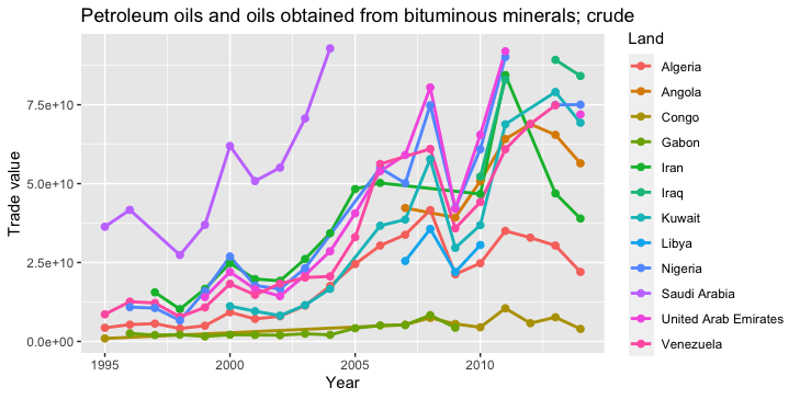
As we can see, some countries has not had oil export for the whole period. We may want to remove some of them, in order to make the table look cleaner. After seeing the table, we want to remove Libya, Iraq and Angola:
04.02 Making a table with less noise
Lorem ipsum dolor sit amet, consectetur adipiscing elit. Sed ut eleifend augue, et pretium turpis. Fusce in tortor a tellus luctus tristique a at metus. Pellentesque in suscipit ipsum. Ut bibendum elit orci, eget efficitur mauris fringilla eget. Aliquam vitae risus lectus. Nam quis ante magna. Nunc hendrerit tellus at tortor dapibus, ut porttitor enim tincidunt. Etiam nisl purus, fermentum sit amet justo ac, lobortis congue ipsum:
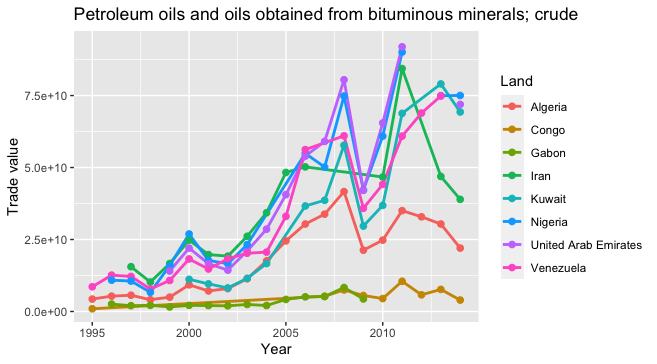
# Subset with different set of countries
# Removing Libya, Iraq and Angola because of lacking data

RSCleanNoNoise <- subset(RSClean, subset = rtTitle == "Algeria" | rtTitle == "Congo" | rtTitle == "Gabon" | rtTitle == "Iran" |             rtTitle == "Kuwait"    | rtTitle == "Nigeria" | rtTitle == "United Arab Emirates" | rtTitle == "Venezuela")

View(RSCleanNoNoise)
Testing new heading here:
Text:
# Visualisation w NoNoise dataframe
# Making the columns into vectors

Year <- c(RSCleanNoNoise$yr)
Value <- c(RSCleanNoNoise$TradeValue)
Land <- c(RSCleanNoNoise$rtTitle)
number 9:
# Converting factors to numerical, and checking the last class, which does not need to be converted

Year <- as.numeric(as.character(RSCleanNoNoise$yr)) # Convert factor to numeric Year
Value <- as.numeric(as.character(RSCleanNoNoise$TradeValue)) # Convert factor to numeric Vekt
class(Land)
And again, the visualisation. Here, Saudi Arabia is is also taken away in order to be able to better see the distribution between the other countries: 10:
FirstVisualisation <- ggplot(RSCleanNoNoise, aes(x = Year , y = Value, group = Land, colour = Land)) +
   geom_line(linewidth=1)

FirstVisualisation <- FirstVisualisation + geom_point(size=2)+
   scale_y_continuous(limits = c(936260544, 92855795003),
                        name = "Trade value")+
   ggtitle(label = "Petroleum oils and oils obtained from bituminous minerals; crude")

FirstVisualisation
11:
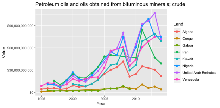
04.03 Making real values on the y- axis
I want the numbers on the y axis to look more normal:
# this is how we do it...

FirstVisualisation + # Modify formatting of axis scale_y_continuous(labels = comma)

FirstVisualisation + # Modify formatting of axis scale_y_continuous(labels = dollar_format())
# Now, the y axis is with dollarsigns
With the result:
04.02:
03.01 Not the most sophisticated plot, but we have to move on
Many things can be said about the formatting of this image, and some of them mught even be unfavourable. However, there are other sites on the web that may learn you how to make beautiful and very sophisticated outputs with RStudio. In this lesson, we are going to focus on breaking down data into a meaninhful regression analysis.
03.02 Etiam tincidunt
“Neque porro quisquam est qui dolorem ipsum quia dolor sit amet, consectetur, adipisci velit…” “There is no one who loves pain itself, who seeks after it and wants to have it, simply because it is pain…”
This is an ordinary paragraph, introducing a block quote.
“It is my business to know things. That is my trade.”
—Sherlock Holmes
04 Lorem ipsum dolor sit amet
Lorem ipsum dolor sit amet, consectetur adipiscing elit. Sed ut eleifend augue, et pretium turpis. Fusce in tortor a tellus luctus tristique a at metus. Pellentesque in suscipit ipsum. Ut bibendum elit orci, eget efficitur mauris fringilla eget. Aliquam vitae risus lectus. Nam quis ante magna. Nunc hendrerit tellus at tortor dapibus, ut porttitor enim tincidunt. Etiam nisl purus, fermentum sit amet justo ac, lobortis congue ipsum. Cras nisl nisi, vehicula ac suscipit vitae, consectetur at ligula. Morbi faucibus dignissim dictum. Phasellus bibendum iaculis tellus, sed vehicula est luctus imperdiet. Pellentesque dictum enim est, at condimentum mauris iaculis et. Nulla posuere congue luctus. Aliquam nec sem pretium massa mollis ornare. Proin vel nulla eu dolor consequat fermentum nec et velit. Ut quis sapien non lacus pretium elementum.
01 Suspendisse consequat sagittis leo at accumsan
02 Suspendisse consequat sagittis leo at accumsan
05 Quisque at finibus orci
Quisque at finibus orci. Suspendisse sit amet magna rutrum nisl tincidunt eleifend. Nulla tempus turpis justo, aliquam viverra ex bibendum at. Praesent accumsan ligula in magna consequat consectetur. Morbi vestibulum tempor odio et commodo. Suspendisse potenti. Suspendisse congue vitae erat eget pellentesque. Donec imperdiet posuere dapibus. Etiam maximus sodales eros, lobortis vulputate mauris commodo ut. Maecenas iaculis sem a tempor tempus. Nulla diam nibh, lacinia non dolor ut, imperdiet aliquet augue. Aenean elit quam, mattis eu ligula a, dapibus sodales nunc. Vivamus a commodo magna, non imperdiet metus.
Suspendisse consequat sagittis leo at accumsan
Suspendisse consequat sagittis leo at accumsan.
Donec dapibus euismod mi ac tempus.
In.hac_habitasse() platea dictumst. Etiam varius nisi eu nunc fringilla ultricies. Ut sapien neque, sollicitudin sed eros id, ornare luctus mauris. Sed ac auctor lorem. Curabitur vitae justo est. Sed quis est at urna malesuada vestibulum sit amet vitae nisi. Vivamus fringilla, nisl quis maximus dignissim, felis justo pulvinar nisi, vitae scelerisque mauris nibh commodo nunc. Nunc eu est nisl. Duis luctus sed sapien eu feugiat. Suspendisse efficitur sagittis neque, non fringilla justo egestas ut. Phasellus posuere pretium est, ac sollicitudin diam egestas in.
Etiam tincidunt
ex ac viverra semper, diam eros laoreet felis, vel maximus purus nunc a augue. Cras ultricies elementum enim. Praesent sed pharetra ipsum. Nullam vel risus tellus. Sed finibus risus at condimentum laoreet. Sed volutpat convallis sapien, id pharetra ante. Quisque sagittis lobortis mattis.
Suspendisse vulputate est vitae nunc porta
Suspendisse vulputate est vitae nunc porta, in tempor sem convallis. Vivamus turpis turpis, imperdiet et viverra et, sodales nec ligula. Nullam ultrices diam sed nisl imperdiet sollicitudin. Quisque id nulla dapibus, tincidunt odio vitae, euismod erat. In in aliquet libero, sed pharetra nisi. Maecenas vel erat pretium, aliquet sapien vitae, ornare neque. Aliquam facilisis, diam vel porttitor tincidunt, tortor eros molestie arcu, nec vulputate enim justo eget nulla. Nam gravida interdum ligula id convallis. Aenean suscipit auctor blandit. Maecenas iaculis lectus in neque mattis, ut hendrerit nunc imperdiet. Sed sed sem sed turpis egestas fringilla. Quisque nec est quis lacus consectetur faucibus tempor vel ex. Integer lobortis augue ac orci vestibulum egestas non blandit diam. Nulla vel lacus nec ex tempus luctus nec eget tortor.
Restetorget
This project has its documentation hosted on Read the Docs: https://readthedocs.org/ The project has a GitHub repository: https://github.com/rasundsbak/rtd-tutorial/tree/3.0.y